There are three broad methods employed for discretizing the governing partial differential equations of a fluid flow:
- Finite Difference Methods (FDM)
- Finite Element Methods (FEM)
- Finite Volume Methods (FVM)
Finite element and finite volume methods (FEM and FVM) are both based on dividing the flow domain into small cells, or volumes. These may possibly take any shape (triangles, quadrilaterals, etc. in 2-D; tetrahedra, prisms, cubes, polyhedra etc. in 3-D). They are thus more suitable for application considering complex flow geometries. Although may be applied to numerically solve both solid mechanics and CFD problems, traditionally FEM found its way mostly to solid mechanics but nonetheless may be applied (sometimes with a very sound basis as in the case of the Galerkin procedure applied to the N.–S. Equations) to fluid problems, FVM tends to be more popular in CFD and generally used in most noticeable major commercial packages. Finite difference schemes can generally be applied to regular-shaped domains using body-fitted grids renders problems of which large grid distortions can not be avoided, as problematic to apply hence not easily applied for very complex flow geometry shapes encountered in most industrial engineering oriented fluid problems. Despite not being generally used in industrial codes, finite difference schemes are useful for introducing the ideas of accuracy, truncation error, stability and boundlessness in a well-defined and fairly transparent way and in the following paragraphs shall do just that. 
The Cell-Reynolds (Cell-Peclet) Problem
In what follows a problem which arises as a consequence of specific properties of solutions to difference equations shall be presented. In contrary to what is often thought, the phenomenon which manifests itself as non-physical oscillation of the numerical solution from one grid point to the next does not arise simply from nonlinearities of Navier–Stokes equations (NSE). Discretized linear equations can exhibit the same kind of behavior as is seen in the NS equation solutions and to appreciate this it shall be presented (as it is usually presented) for the following 1-D steady-state convection-diffusion problem, a simplification homogeneous Burgers’ equation, one of the few nonlinear equations to possess an exact solution: ![]() The simplification to the Burgers’ equation shall be quite significant as to illustrate the fact that nonlinearities are not the cause the linearized steady-state form shall be treated:
The simplification to the Burgers’ equation shall be quite significant as to illustrate the fact that nonlinearities are not the cause the linearized steady-state form shall be treated:  where U is a known constant.
  Discretize the simplified equation with centered differences to obtain:
  where h is the discretization step size. Intentionally multiplying by h/U leaves this in the form:
  We now define the cell-Reynolds number as:
 The starting point toward understanding the cell-Re problem stems from a property of elliptic and parabolic differential equations known as the maximum principle. Starting from the basic fact from calculus that if a function f(x) satisfies f” > 0 on an interval [a, b], then it can only achieve its maximum on the boundary of that interval. For partial differential equations, the same idea allows to draw very useful conclusions from the properties of the solutions and the domain of a given problem and it shall allow a quick view on the properties of linear discretization of such entities. We shall start by defining L as an elliptic linear partial differential operator (as the Laplacian operator for example). Formally for an elliptic operator with a bounded domain we shall write:
  and the boundary condition satisfies:
  Then the maximum principle states that the maximum and minimum values of u occur on the boundary. Since it’s difference approximations are our concern, it shall be stated that a similar principle exists for difference approximations to elliptic equations of the following general form:
  To guarantee such a maximum principle for discretizations two conditions must be satisfied:
- Non-negativity:

- diagonal dominance:

These requirements are not dependent upon the spatial dimension of the problem or on the specific formulation for differencing involved in the construction of the approximation. In particular, they are sufficient even on unstructured grids. We shall observe the discretized version of the maximum principle in a local sense rather than the whole domain. Specifically, if we consider placing a boundary around each grid, the maximum principle implies that the grid function value at the point (i, j) cannot exceed that of any of its nearest neighbors, and because there is a corresponding minimum principle, the grid-function value cannot be lower than that of any neighbor, meaning it cannot oscillate from point to point. Returning to the discretized linear (steady-state) advection-diffusion and using the definition for cell-Reynolds: we obtain the following: ![]() and rewrite in the following form:
and rewrite in the following form:  What is obvious from the above form is that for |Reh| > 2 the non-negativity condition shall not be satisfied, which in turn might mean a failure to meet the maximum principle and consequent local extremum in the interior of the solution. In numerical computations involving transport equations the symptom of this problem is non-physical oscillation of the numerical solution from one grid point to the next.
Some notions from the mathematical theory of difference equations
In what follows which shall be referred as disclosed Parenthetically, some notions on the order of a difference and the number of independent solutions to a linear difference equation shall be discussed. The first notion is actually a definition relating the order of a difference equation to the difference between the highest and lowest subscripts appearing on its terms. In the above equation it’s simply:  In the second notion we shall refer to a theorem claiming that the number of independent solutions to a linear difference equation is equal to its order. Solving analytically linear difference equation is very similar to the route taken for linear differential equations, i.e. we shall consider a linear difference equation of which form is representative to the above equation (meaning second order but in general form):
  As conducted similarly for differential equation we may obtain a second order characteristic equation:
  We know how to solve exactly such polynomial equations (at least up to fourth-order difference equations), and for the above we get the following solution:
  Then the independent solution to the second order (linear) difference equation becomes:
  for i=1,2,…N as N being the number of discrete points in our domain. We complete our understanding with another theorem stating that the general solution to the (general form) linear difference equation is a linear combination of the independent solutions given above, meaning:
  where the constants are to be evaluated through boundary (or depending on the nature of the problem – initial) conditions.
Manifestation of the cell-Reynolds problem from a rigorous view
We see that the linearized steady-state model for the Burger’s equation we have taken on has an identical discretized form to the parenthetically disclosed above general form linear difference equation and thus for our case we find the following solution for the characteristic equation:
 and
and 
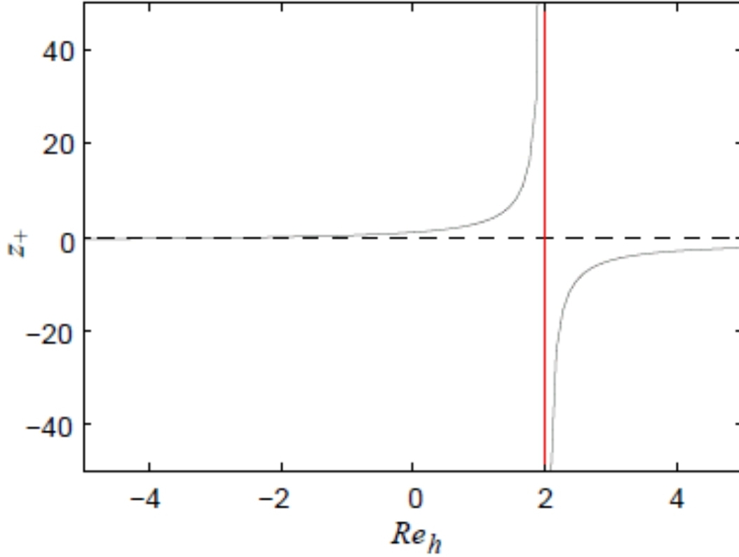
Plotting values of z+ against the cell-Reynolds we see the following dependence: 
Now before concluding our remarks in an organized manner, it is important to note that such an issue is one of those which stand in the basis of CFD understanding and as written above, such a phenomena in numerical modeling is a consequence of specific properties of solutions to difference equations rather than simply from nonlinearities of NSE.
We then conclude with the following observations:
- For the case of centered-difference approximation to our equation z+ first becomes negative when the cell-Reynolds exceeds 2 and that z+ is going to ∞ as the cell-Reynolds is approaching 2 from boat sides and this is in accordance with the heuristic analysis based on the maximum principle and now derived purely from the mathematical theory of difference equations. This is an important note as it means that the cell-Reynolds restriction for centered difference approximation is more than a physical argument such as the appeal to flow direction to suggest the inadequacy of the specific approximation.
- As we see from the definition of cell-Reynolds, i.e.: having the discretization step size h in the definition points us to the fact that failure to maintain a cell-Reynolds which does not exceed 2 is a form of under resolution (decrease the discretization step size h and the cell-Reynolds shall decrease accordingly). Although this is different from under resolution in the usual sense, meaning insufficient grid points to represent the solution to the differential equation but rather an undesirable property (wiggles) in the solution for linear difference equations, the effect is quite similar and as such both may be treated in the same manner.
- An interesting observation from the above z+ Vs. cell-Reynolds plot is that in general the situation is much worse when the cell-Reynolds is positive rather than negative and since the velocity U is the only factor in the cell-Reynolds definition which may be either negative or positive it is suggested that we might evidently find the cell-Reynolds problem more severe for high-speed forward flow than in reversed flows. Nevertheless it is important to note that eventually, the actual numerical solution for the difference equation: is dependable upon the constants (c1 and c2) which in their turn are set by boundary conditions. This means that for certain combinations of boundary conditions, for example when c2>>c1, the cell-Reynolds problem might not be particularly significant even though the basic centered-difference approximation may have violated the discrete maximum principle. On the other hand, we should keep in mind that in the above case c2>>c1, as the cell-Reynolds effects will be significant only for cell-Reynolds number slightly greater than two, even in high-speed flows where the absolute value of the cell-Reynolds is much grater than two, it is still likely that the absolute value of the cell-Reynolds will be only slightly greater than two in specific regions ( for example near solid boundaries, in some regions of shear layers and in the cores of vortices). This leads us to conclude that the cell-Reynolds problem might be encountered in any simulation that is even slightly under resolved.
- In multi-dimensional flow fields all components of velocity (and their associated boundary conditions) contribute hence there is no more one single cell-Reynolds per grid point but a distinct value for each separate advective term of the momentum equations. As the contribution in multi-dimensional flow fields (sometimes manifests itself in ways leading to local cancellations, it is considerably more complicate to get a sense the overall situation of under resolve grid spacing whilst still keeping the mesh affordable from a computation resources point of view.
Remedies for the Cell-Reynolds Problem
There are some several widely-used ways to treat the cell-Reynolds problem. In what follows some popular approximations such as first and second order upwinding and QUICK shall be discussed. ANSYS Fluent (and nearly all notable commercial codes) provides means to employ these specific approximations including the standard centered difference approximation.
- First-Order Upwind: This is probably the first approach to treat the cell-Reynolds problem, originating from S. V. Patankar (father to the original SIMPLE algorithm). Patankar had taken an ad-hoc “physical reasoning” arguing that as it is clear from the representation of centered difference approximation to the velocity gradient both upstream and downstream flow behavior are sensed. Hence a least biased difference approximation, using only information carried in the flow direction in its simplest form is offered. After employing the simplification as in the above procedure we arrive to the following form:
 This difference equation satisfies non-negativity and hence the extermum conditions for difference equations. On the other hand, the specific approximation’s shortcoming may be viewed by performing a simple procedure. We shall take the non-dimensional for of the linearized steady-state Burger’s equation:
  and remember that upwind difference approximation we employ the following backward difference for the velocity gradient at grid i:
  expansion of u at grid point i-1 around grid i yields:
  which may then be replaced to the linearized steady-state Burger’s equation above to achieve the following form:
  we shall write the above equation as:
  this equation is termed the modified equation and it is actually it rather than the original partial differential equation which is solved to second order accuracy instead of the first order accuracy the discretization implies. In the above equation, Re* is an effective Reynolds defined as:
  What is clear from the above analysis is that first-order upwind approximation effectively increases the coefficient of the diffusion (!), a phenomena often called numerical diffusion.
- Second-Order Upwind: Here we follow (without the elaboration as taken for the first-order upwind) a reference from W. Shyy (1985) assisted by other pointed out references. The form of the linearized steady-state Burger’s equation after applying second-order one-sided differences:
 We note the switching applied in order to keep the difference into the flow direction.We observe and conclude the following important notions:
- As is obvious, the discretization is second-order accurate. This means a five-point discrete representation, resulting in a more complicated matrix structure if implicit time stepping is employed in the solution algorithm.
- As it turns out the leading terms of the modified equation are those of the original equation which means that the physics is not compromised by this approximation.
- Because the second order upwind differencing connects two upstream nodes, it is necessary to follow special practices for the finite difference nodes adjacent to a boundary; otherwise reference will have to be made to a value outside the flow domain. There are two popular techniques to deal with that notion. M. Atias et al. (“Efficiency of Navier-Stokes Solver” – 1977) proposed switching back to first order upwind differencing for cells adjacent to a solid boundary. A different route proposed by W. Shyy and S. M. Correa (“A Systematic Comparison of Several Numerical Schemes for Complex Flow Calculations” – 1985) is to use the hybrid formulation near the boundaries. The hybrid formulation at boundaries is the same as the upwind formulation except that when the boundary cell -Reynolds number is less than two, central differencing is used.
- the roots of the corresponding difference equation are all non-negative, independent of the value of cell Re. Hence, formally, there is no cell-Re restriction associated with this approximation.
- We further note that referring to the theoretical difference equation analysis above neither non-negativity of the difference equation coefficients nor diagonal dominance hold for this scheme, implying that it does not satisfy a maximum principle in the sense described earlier. This reflects the fact that those conditions pose satisfactory but not necessary conditions meaning that in order to not draw erroneous conclusions about the cell-Reynolds problem more emphasis should be placed on finding the solutions to the difference equation.
- Finally, as guidance for whether to make use of a second rather than a first order approximation we shall add that When the flow is aligned with the flow gradients (e.g., laminar flow in a rectangular duct modeled with a quadrilateral or hexahedral grid) the first-order upwind discretization may be acceptable. When the flow is not aligned with the flow gradients (i.e., when it crosses the grid lines obliquely), however, first-order convective discretization increases the numerical discretization error (numerical diffusion).This is quite an important topic of which there is a consensus among CFD practitioners, i.e. the impact of alignment of flow gradients on phenomena like numerical diffusion an dispersion. Not to delve to deep into the topic, looking at the pure convection equation:

The above PDE’s modified equation (the PDE which the exact solution to the discretized equations satisfies) is:

Meaning that the numerical behavior of the discretization scheme largely depends on the relative importance of dispersive and dissipative effects, specifically, a low order scheme along with a mesh which is not aligned with the flow’s gradients will tend to smear all over the place:

Quad Vs. tri mesh: contours of axial velocity for the case of inviscid co-flow jet There is of course no benefit in this aspect when there is no dominant flow gradient direction:

Quad Vs. tri mesh: contours of temperature for inviscid flow Poly mesh would not be as aligned with the flow gradients for very simple flows such as the above, but due to the multiplicity of faces it has 6 optimal direction (if it has 12 faces) in contrast with hex which have 3 optimal faces, it may be more accurate than hex mesh for recirculating flows even for those which seem optimal for hex as they have a cartesian domain such as the qubic lid-driven cavity:

Referring to mesh methodologies we then add that for triangular and tetrahedral grids, since the flow is never aligned with the grid, you will generally obtain more accurate results by using the second-order discretization. For quad/hex grids, you will also obtain better results using the second-order discretization, especially for complex flows. For a simple flow that is aligned with the flow gradients (e.g., laminar flow in a rectangular duct modeled with a quadrilateral or hexahedral grid), the numerical diffusion will be naturally low, so you can generally use the first-order scheme instead of the second-order scheme without any significant loss of accuracy. For most cases, you will be able to use the second-order scheme from the start of the calculation. In some cases, however, you may need to start with the first-order scheme and then switch to the second-order scheme after a few iterations. For example, if you are running a high-Mach-number flow calculation that has an initial solution much different than the expected final solution, you will usually need to perform a few iterations with the first-order scheme and then turn on the second-order scheme and continue the calculation to convergence. In summary, while the first-order discretization generally yields better convergence than the second-order scheme, it generally will yield less accurate results, especially on tri/tet grids, concluding that strong emphasis should be taken to control convergence. ANSYS Fluent allows for various of direct ways to do just that by Modifying Algebraic Multigrid Parameters, Setting FAS Multigrid Parameters and Modifying Multi-Stage Time-Stepping Parameters for example.
- QUICK: The quadratic upstream interpolation for convective kinematics scheme of B. P. Leonard (“A stable and accurate convection modelling procedure based on quadratic upstream interpolation” – 1979) is one of the most popular techniques for remedying the cell-Reynolds problem. The form of the linearized steady-state Burger’s equation after applying second-order one-sided differences for the QUICK approximation is as follows:
 For the one-dimensional domain shown in the figure the Φ value at a control volume face is approximated using three-point quadratic function passing through the surrounding nodes and one other node on upstream side:
  We observe and conclude the following important notions:
- Although the original intention by B. P. Leonard to produce a method with third order accuracy this was actually with respect to a location in the grid stencil that did not correspond to any grid point. It is most important to note that in contrast to what is frequently thought QUICK is second-order accurate.
- We note the switching applied in order to keep the difference into the flow direction only in QUICK it is referred to as upwind biased as the stencil extends to both downstream and upstream of a specific grid point.
- As for the second-order upwind approximation neither non-negativity of the difference equation coefficients nor diagonal dominance hold for this scheme, implying that it does not satisfy a maximum principle in the sense described earlier but in contrast to the former it has a cell-Reynolds restriction:

- Although the above restriction there is a general favorable experience regarding the cell-Reynolds problem. Nevertheless, although being a very accurate scheme, in regions with strong gradients, overshoots and undershoots can occur lead to stability problems in the calculation.
Practical guidelines
- When the flow is aligned with the flow gradients (for example, laminar flow in a rectangular duct modeled with a quadrilateral or hexahedral mesh) the first-order upwind discretization may be acceptable, otherwise, (as is the case when the flow crosses the mesh lines obliquely), first-order discretization increases the numerical discretization error through numerical diffusion. For triangular and tetrahedral meshes, since the flow is never aligned with the flow gradients, more accurate results shall be obtained by using the second-order discretization. Keep in mind (especially for complex flows) that even for hex meshes, you will also obtain better results using the second-order discretization.
- For most cases, it is possible to use the second-order scheme from the start of the calculation. There are some cases, however, where it is preferable to perform an initial few iterations with the first-order scheme and then switch to the second order (high-Mach-number flow for example).
- The QUICK scheme may provide better accuracy than the secondorder scheme for rotating or swirling flows. The QUICK scheme is applicable to hexahedral meshes. An alternative scheme, the 3rd order MUSCL scheme, may be used on all types of meshes. Keep in mind howeever that the second-order upwind scheme is sufficient in most cases and the QUICK scheme will not provide significant improvements in accuracy.
We shall close the discussion about the cell- Reynolds problem with a summary table regarding the approximations presented and reference to their cell-Reynolds restriction: 


Great article. Always knew upwinding is required to discretise the convection term, in order to obtain monotonic solutions but to see it from a mathematical perspective was interesting.
This is a useful post that needs to be shared. Although it doesn’t necessarily contain ‘new’ information it nevertheless should be published in a journal. I think there are still people who think hexas with a 2nd order central scheme is right way to solve general cfd problems.
Yes